
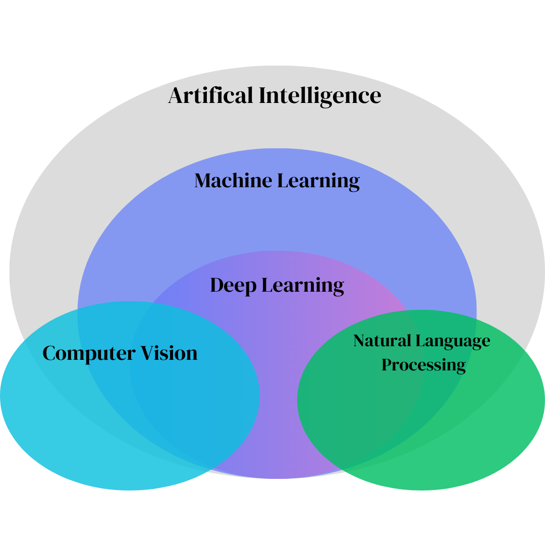
Overview of Computer Vision
Overview of Computer Vision
Computer vision (CV) is the science of teaching machines to interpret and understand visual data. Since 2012 (ILSVRC, AlexNet), CV has shifted from algorithmic, rule-based systems to use data-driven, optimization-based systems.
The core of modern CV lies in the mathematical formalization of the learning problem, where a model learns a function $f: \mathcal{X} \rightarrow \mathcal{Y}$ that maps an input space of images $\mathcal{X}$ to an output space of predictions $\mathcal{Y}$.
For display equations:
$$ \mathcal{L}_{CE}(\theta) = -\sum_{i=1}^{N} \sum_{k=1}^{K} y_{i,k} \log p_{i,k} $$Computer vision (CV) is the science of teaching machines to interpret and understand visual data. Since 2012 (ILSVRC, AlexNet), CV has shifted from algorithmic, rule-based systems to use data-driven, optimization-based systems.
The core of modern CV lies in the mathematical formalization of the learning problem, where a model learns a function $f: \mathcal{X} \rightarrow \mathcal{Y}$ that maps an input space of images $\mathcal{X}$ to an output space of predictions $\mathcal{Y}$.
Computer vision (CV) is the science of teaching machines to interpret and understand visual data. Since 2012 (ILSVRC, AlexNet), CV has shifted from algorithmic, rule-based systems to use data-driven, optimization-based systems.
The core of modern CV lies in the mathematical formalization of the learning problem, where a model learns a function $f: \mathcal{X} \rightarrow \mathcal{Y}$ that maps an input space of images $\mathcal{L}_{X}$ to an output space of predictions $\mathcal{Y}$.
Mathematical Formalism of Core CV Tasks
At its heart, a CV task is an optimization problem where the goal is to find a set of model parameters $\theta$ that minimize a loss function $\mathcal{L}_{CE}$ .
Image Classification
Assigning a single or multiple labels to an image, at an image level (e.g., image contains cat vs. dog).
Example:
This is a multiclass classification problem. Given an image $\mathbf{x} \in \mathbb{R}^{H \times W \times C}$ (height, width, channels), the model outputs a probability distribution $\mathbf{p} = [p_1, \dots, p_K]$ over $K$ classes. A standard loss could be cross-entropy, MSE, etc. Here's standard cross-entropy loss:
$$ mathcal{L}_{CE}(\theta) = -\sum_{i=1}^{N} \sum_{k=1}^{K} y_{i,k} \log p_{i,k} $$where $N$ is the number of samples, $y_{i,k}$ is a one-hot encoded ground-truth label, and $p_{i,k}$ is the predicted probability. The model parameters $\theta$ are updated using stochastic gradient descent (SGD) or its variants.
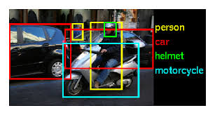
Object Detection
This task is a composite problem involving both classification and regression. For each object, the model predicts a class label and a bounding box. The total loss is typically a weighted sum of two components:
$$ \mathcal{L}_{Total} = \mathcal{L}_{cls} + \lambda \mathcal{L}_{loc} $$Here, $\mathcal{L}_{cls}$ is a classification loss, and $\mathcal{L}_{loc}$ is a regression loss (e.g., L1 loss or IoU loss) for the bounding box coordinates. The parameter $\lambda$ balances the two terms.
Segmentation (Semantic and Instance)
These are pixel-level classification problems. The loss is often a pixel-wise cross-entropy loss or a Dice loss, which measures the overlap between the predicted and ground-truth masks.
Theoretical Underpinnings of Architectures
The architectural choice defines the function $f(\mathbf{x}; \theta)$ and the inductive biases it possesses.
Convolutional Neural Networks (CNNs)
The core of a CNN is the convolutional layer. This operation is defined by a convolution integral (or summation for discrete data):
$$ (I * K)(i, j) = \sum_{m} \sum_{n} I(i-m, j-n) K(m, n) $$The key theoretical principles of CNNs are:
- Parameter Sharing: A single kernel is applied across the entire image.
- Equivariance to Translation: Shifting an object results in a corresponding shift in the feature map.
- Hierarchy of Features: Deeper layers learn more complex, abstract features.
Feature Extraction — What to Look For
Features with high variance
Non-correlated features
Discriminative
Orthogonal & unit vectors
Vision Transformers (ViTs)
ViTs discard convolutions in favor of the attention mechanism. The core is the multi-head self-attention layer:
$$ \text{Attention}(Q, K, V) = \text{softmax}\left(\frac{QK^T}{\sqrt{d_k}}\right)V $$Unlike CNNs, which have a local receptive field, the self-attention mechanism allows a ViT to model global dependencies between all patches, regardless of their spatial distance.
Learning Paradigms and Theoretical Concepts
Self-Supervised Learning (SSL)
This paradigm generates supervision from the data itself. The core idea is to train a model to solvve a pretext task>.
- Contrastive Learning: Models learn to pull together (in an embedding space) different augmented views of the same image while pushing apart views of different images.
- Masked Image Modeling (MIM): The model masks a high percentage of image patches and trains to reconstruct the missing pixels.
Generative Models (GANs & Diffusion)
These models learn the underlying probability distribution of the training data $p_{data}(\mathbf{x})$ to generate new samples.
- Generative Adversarial Networks (GANs): This is a minimax game with the value function: $$ \min_G \max_D V(D, G) = \mathbb{E}_{\mathbf{x} \sim p_{data}(\mathbf{x})}[\log D(\mathbf{x})] + \mathbb{E}_{\mathbf{z} \sim p_z(\mathbf{z})}[\log(1 - D(G(\mathbf{z})))] $$
- Diffusion Models: These models learn to reverse a gradual, iterative process of adding Gaussian noise to an image. This process can be mathematically defined as a Markov chain.
Regularization and Optimization
Regularization techniques are mathematical tools used to prevent overfitting and improve model generalization.
- L2 Regularization (Weight Decay): Adds a penalty term to the loss function that is proportional to the square of the magnitude of the weights.$$ \mathcal{L}_{new}(\theta) = \mathcal{L}_{original}(\theta) + \lambda \sum_{i} \theta_i^2 $$
- Dropout: Randomly "drops out" neurons during training, which acts as a form of ensemble learning.
- Data Augmentation: Expands the training data by applying transformations, forcing the model to learn representations that are invariant to these changes.
Overfitting Scenario
Train on 20 samples → good results
New dataset → poor performance
Reasons:
Too many free parameters vs training data
Overfitting → memorization
Inadequate complexity
Unbalanced data
Unnormalized data
Fix:
More data
Regularization
Data augmentation
Underfitting
Model too simple to capture patterns
Fix:
Increase complexity
Add features
More epochs
Fully Connected Neural Network Design
Linear vs Non-linear
Activations must be non-linear to learn complex mappings
Loss must be differentiable
Activation Functions
tanh vs ReLU
ReLU:
𝑓 ( 𝑧 )
max ( 0 , 𝑧 ) f(z)=max(0,z) ∂ 𝑓 ∂ 𝑧
1 if 𝑧
0 , 0 otherwise ∂z ∂f
=1 if z>0,0 otherwise
No vanishing gradient
Can cause exploding gradient
tanh:
Symmetric output
Faster convergence early in training
Computer Vision
Overview of Computer Vision
Core concepts in computer vision and machine learning
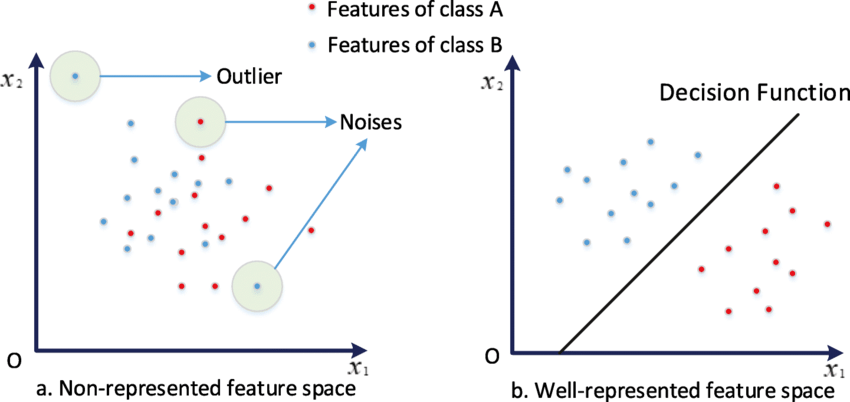
History of Computer Vision
How computer vision evolved through feature spaces
ImageNet Large Scale Visual Recognition Challenge
ImageNet's impact on modern computer vision
Region-CNNs
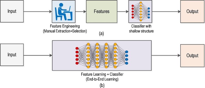
Traditional ML vs modern computer vision approaches
Distributed Systems
Overview of Distributed Systems
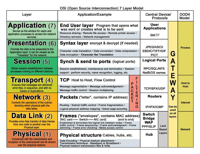
Fundamentals of distributed systems and the OSI model

Distributed Systems Architectures
Common design patterns for distributed systems
Dependability & Relevant Concepts
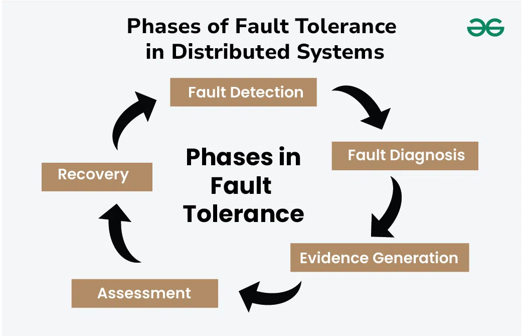
Reliability and fault tolerance in distributed systems
Marshalling
How data gets serialized for network communication
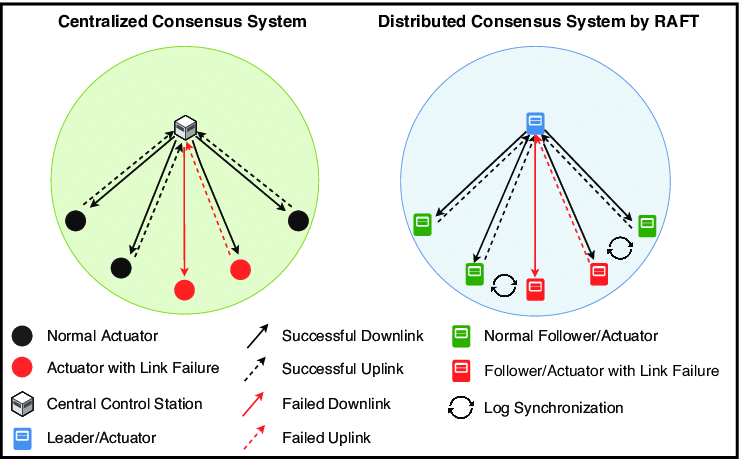
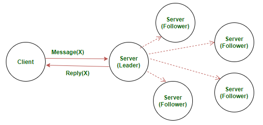
RAFT
Understanding the RAFT consensus algorithm
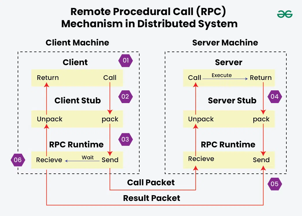
Remote Procedural Calls
How RPC enables communication between processes
Servers
Server design and RAFT implementation
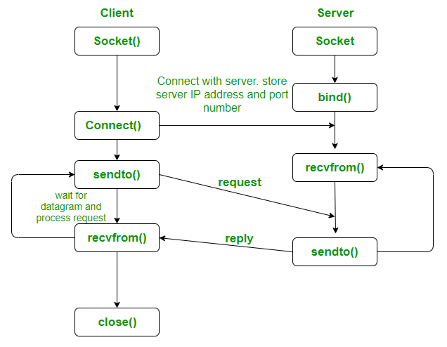
Sockets
Network programming with UDP sockets
Machine Learning (Generally Neural Networks)
Anatomy of Neural Networks
Traditional ML vs modern computer vision approaches

LeNet Architecture
The LeNet neural network
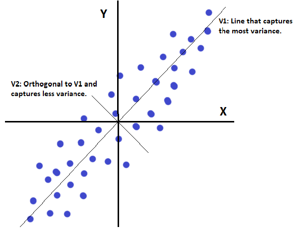
Principal Component Analysis
Explaining PCA from classical and ANN perspectives
Cryptography & Secure Digital Systems
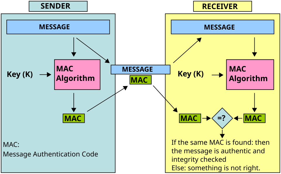
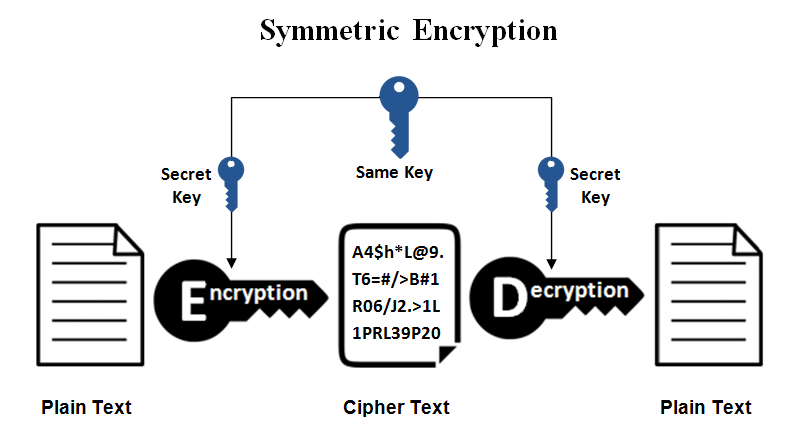
Symmetric Cryptography
covers MAC, secret key systems, and symmetric ciphers
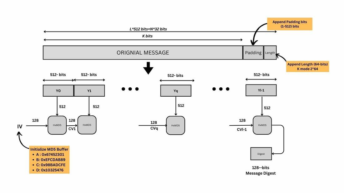
Hash Functions
Hash function uses in cryptographic schemes (no keys)
Public-Key Encryption
RSA, ECC, and ElGamal encryption schemes
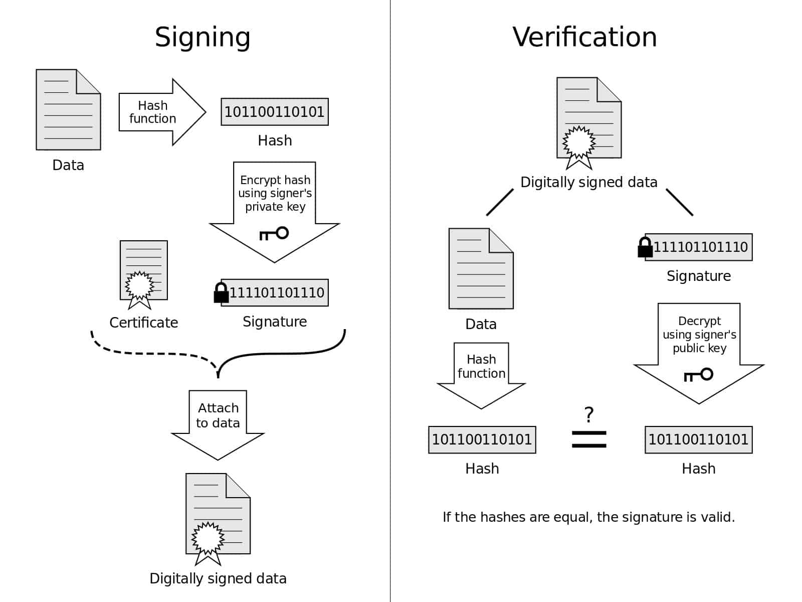
Digital Signatures & Authentication
Public-key authentication protocols, RSA signatures, and mutual authentication

Number Theory
Number theory in cypto - Euclidean algorithm, number factorization, modulo operations
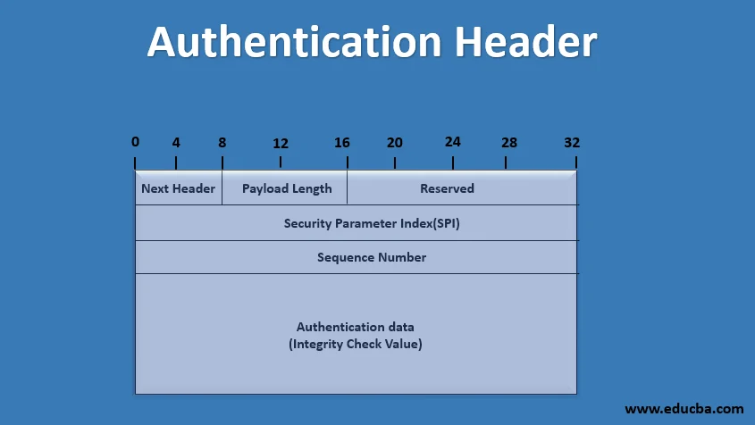
IPSec Types & Properties
Authentication Header (AH), ESP, Transport vs Tunnel modes