
PCA (Principal Component Analysis)
Table of Contents
- Overview
- Orthogonal
- Dimensionality Reduction
- Key PCA Notes
- Benefits of PCA
- Component Selection
- Statistical Approach
- PCA Example
- ANN Approach (PCA Network)
Overview
- Multiple features combined into 1 feature → that feature has more data → combining existing features results in a single feature
- Hard for 3D → visualizing beyond 3 dimensions is impossible for humans
- You can choose a dimension in the direction of smallest change → remove dimensions with low variance (noise)
- Apply orthogonal transformation & reduce dimensionality → rotate axes to align with variance
- PCA is unsupervised learning → no labeled data required
- PCA decorrelates data → removes linear correlations between features
Result:
- Fewer features with high variance → keep most important information
- Linearly independent → no redundancy between new features
- Significantly different → each principal component captures unique variance
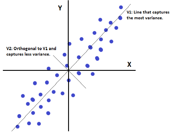
Orthogonal
- $A \cdot B = 0$ → perpendicular vectors
- $A \cdot A = 1$ → unit length (normalized)
- Orthogonal features → principal components are perpendicular to each other
Dimensionality Reduction
- 3 domains → 2 domains $x = [x_1, x_2, x_3]$
Where $W$ is the transformation matrix with rows $w_1, w_2$ (principal components)
Aspects
- If vectors are independent, they are uncorrelated → independence implies uncorrelation
- If vectors are uncorrelated, they aren’t necessarily independent → uncorrelation doesn’t guarantee independence
- In direction of highest variance:
- Vectors are orthogonal → perpendicular to each other
- Dot product = 0 → no correlation
- No information overlap → each captures unique variance
- Loss minimized → reconstruction error is smallest
- Can’t completely remove $x_1, x_2$ → find new variance to adapt / merge $x_1, x_2$ → project onto lower-dimensional space while preserving maximum variance
Benefits of PCA
- Dimensionality reduction with minimal loss → retain most important information
- Noise reduction → remove components with low variance (noise)
- Improved visualization → reduce to 2D or 3D for plotting
- Reduces collinearity → eliminates correlation between features
- More efficient computation → fewer features = faster processing
- Improved model performance → reduces overfitting and computational cost
Statistical Approach
- Center data onto variance $x_i - \text{mean vector}$ → shift origin to center of data
- Find covariance matrix → captures how features vary together
- Find eigenvectors + eigenvalues → directions and magnitudes of variance
- Trace = sum of all eigenvalues → total variance in data
- Order eigenvectors by largest eigenvalue → $w_i$ is the largest eigenvector for that dimension → first PC explains most variance
- Calculate explained variance:
→ % of characteristics from that vector input → how much variance this PC captures
Eigenvalue Example
Given points: $(4,0), (0,1), (-4,0), (0,-1)$ what are the eigenvalues and eigenvectors?
Steps:
- Compute mean
- Compute covariance
- Solve:
Answers:
Eigenvalues:
- $\lambda_1 = 8$
- $\lambda_2 = \frac{1}{2}$
Eigenvectors:
- $v_1 = [1, 0]$
- $v_2 = [0, 1]$
Solutions
PCA Eigenvalue Example - Complete Solution
Given points: $(4,0), (0,1), (-4,0), (0,-1)$ what are the eigenvalues and eigenvectors?
Step 1: Compute Mean
$$ \bar{x} = \frac{1}{4}[(4,0) + (0,1) + (-4,0) + (0,-1)] = \frac{1}{4}(0,0) = (0,0) $$The mean is already at the origin, so the data is centered.
Step 2: Compute Covariance Matrix
The covariance matrix is:
$$ C_x = \frac{1}{N} \sum_{i=1}^{N} (x_i - \bar{x})(x_i - \bar{x})^T $$Since $\bar{x} = (0,0)$:
$$ C_x = \frac{1}{4}\left[\begin{bmatrix} 4 \\ 0 \end{bmatrix}\begin{bmatrix} 4 & 0 \end{bmatrix} + \begin{bmatrix} 0 \\ 1 \end{bmatrix}\begin{bmatrix} 0 & 1 \end{bmatrix} + \begin{bmatrix} -4 \\ 0 \end{bmatrix}\begin{bmatrix} -4 & 0 \end{bmatrix} + \begin{bmatrix} 0 \\ -1 \end{bmatrix}\begin{bmatrix} 0 & -1 \end{bmatrix}\right] $$$$ C_x = \frac{1}{4}\left[\begin{bmatrix} 16 & 0 \\ 0 & 0 \end{bmatrix} + \begin{bmatrix} 0 & 0 \\ 0 & 1 \end{bmatrix} + \begin{bmatrix} 16 & 0 \\ 0 & 0 \end{bmatrix} + \begin{bmatrix} 0 & 0 \\ 0 & 1 \end{bmatrix}\right] $$$$ C_x = \frac{1}{4}\begin{bmatrix} 32 & 0 \\ 0 & 2 \end{bmatrix} = \begin{bmatrix} 8 & 0 \\ 0 & \frac{1}{2} \end{bmatrix} $$Step 3: Solve for Eigenvalues
$$ \det(C_x - \lambda I) = 0 $$$$ \det\begin{bmatrix} 8-\lambda & 0 \\ 0 & \frac{1}{2}-\lambda \end{bmatrix} = 0 $$$$ (8-\lambda)\left(\frac{1}{2}-\lambda\right) = 0 $$Eigenvalues:
- $\lambda_1 = 8$ (largest eigenvalue → most variance along x-axis)
- $\lambda_2 = \frac{1}{2}$ (smaller eigenvalue → less variance along y-axis)
Step 4: Solve for Eigenvectors
For $\lambda_1 = 8$:
$$ (C_x - 8I)v_1 = 0 $$$$ \begin{bmatrix} 0 & 0 \\ 0 & -\frac{15}{2} \end{bmatrix}\begin{bmatrix} v_{11} \\ v_{12} \end{bmatrix} = \begin{bmatrix} 0 \\ 0 \end{bmatrix} $$This gives $v_{12} = 0$, so $v_1 = [1, 0]$ (direction of maximum variance)
For $\lambda_2 = \frac{1}{2}$:
$$ (C_x - \frac{1}{2}I)v_2 = 0 $$$$ \begin{bmatrix} \frac{15}{2} & 0 \\ 0 & 0 \end{bmatrix}\begin{bmatrix} v_{21} \\ v_{22} \end{bmatrix} = \begin{bmatrix} 0 \\ 0 \end{bmatrix} $$This gives $v_{21} = 0$, so $v_2 = [0, 1]$ (direction of minimum variance)
Interpretation
- First principal component ($v_1 = [1,0]$): Horizontal direction with variance = 8
- Second principal component ($v_2 = [0,1]$): Vertical direction with variance = 0.5
- The data varies much more along the x-axis than the y-axis (8 vs 0.5)
- Total variance = $8 + 0.5 = 8.5$
- PC1 explains $\frac{8}{8.5} \approx 94.1%$ of the variance
- PC2 explains $\frac{0.5}{8.5} \approx 5.9%$ of the variance
ANN Approach (PCA Network)
- No hidden layers → direct input-to-output mapping
- Initialize with random weights → weights used to calculate eigenvectors → learns PCs through training
- Output is weighted sum of inputs $y = x_i \cdot w_j$ → linear transformation
- Each output node has a weight vector $w_i$ → one row of transformation matrix $W$ → learns one principal component
Update Rule:
$$ \Delta w_i = \eta y_i x_i^T - k_i w_i \quad (\text{L2 regularization}) $$→ Hebbian learning term $\eta y_i x_i^T$ strengthens weights based on correlation → Regularization term $k_i w_i$ prevents weights from growing unbounded
Iteration:
- Normalize weights: $|w| = 1$ → keep weights on unit sphere
- Direction of $w$ is highest eigenvalue vector → converges to principal component
- $\lambda = E[y^2] = \frac{1}{N} \sum y_i^2$ → variance captured by this PC
- Lies in direction of maximum variance → minimum loss → optimal dimensionality reduction
Computer Vision
Overview of Computer Vision
Core concepts in computer vision and machine learning
History of Computer Vision
How computer vision evolved through feature spaces
ImageNet Large Scale Visual Recognition Challenge
ImageNet's impact on modern computer vision
Region-CNNs
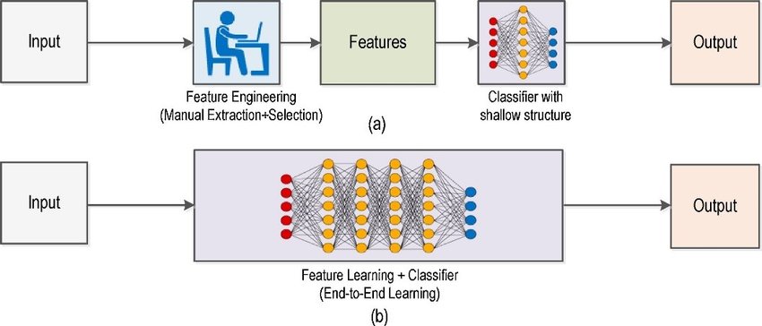
Traditional ML vs modern computer vision approaches
Distributed Systems
Overview of Distributed Systems
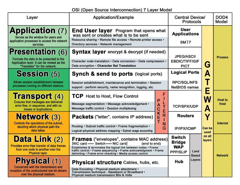
Fundamentals of distributed systems and the OSI model
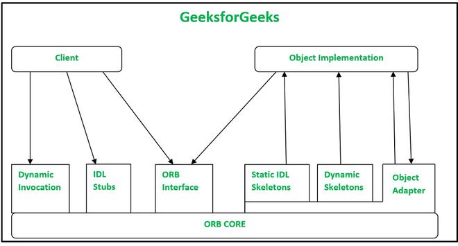
Distributed Systems Architectures
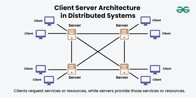
Common design patterns for distributed systems
Dependability & Relevant Concepts
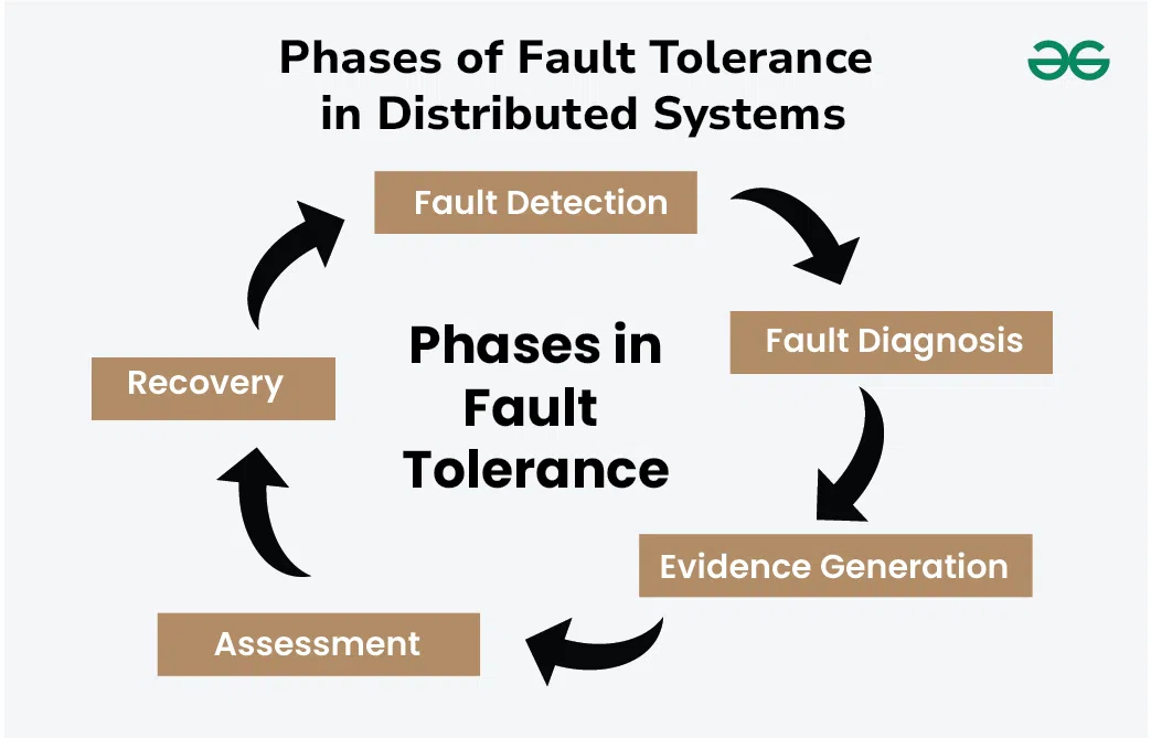
Reliability and fault tolerance in distributed systems
Marshalling
How data gets serialized for network communication
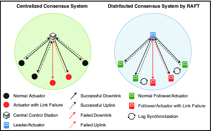
RAFT
Understanding the RAFT consensus algorithm
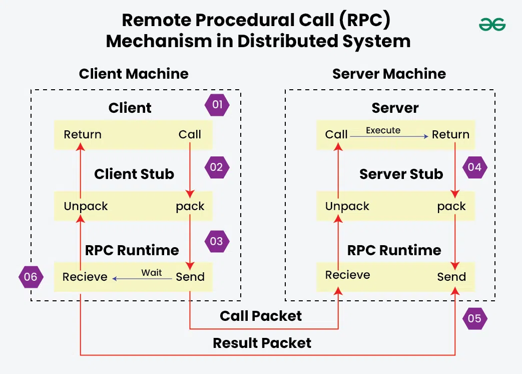
Remote Procedural Calls
How RPC enables communication between processes
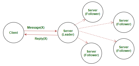
Servers
Server design and RAFT implementation
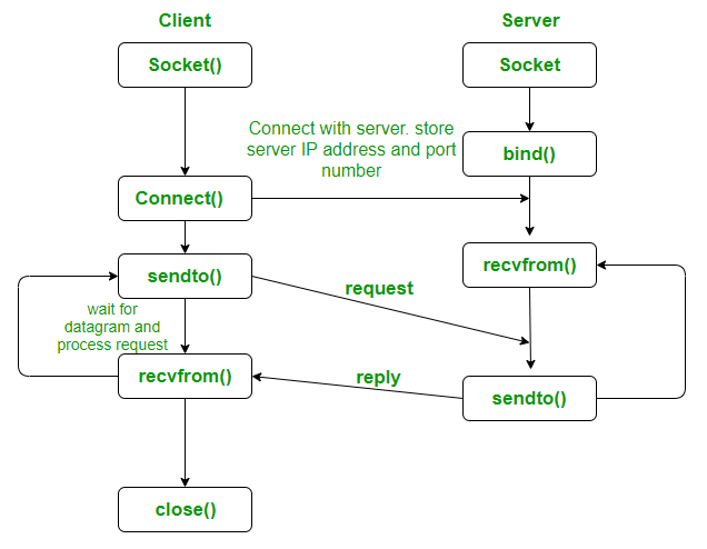
Sockets
Network programming with UDP sockets
Machine Learning (Generally Neural Networks)
Anatomy of Neural Networks
Traditional ML vs modern computer vision approaches

LeNet Architecture
The LeNet neural network
Principal Component Analysis
Explaining PCA from classical and ANN perspectives
Cryptography & Secure Digital Systems
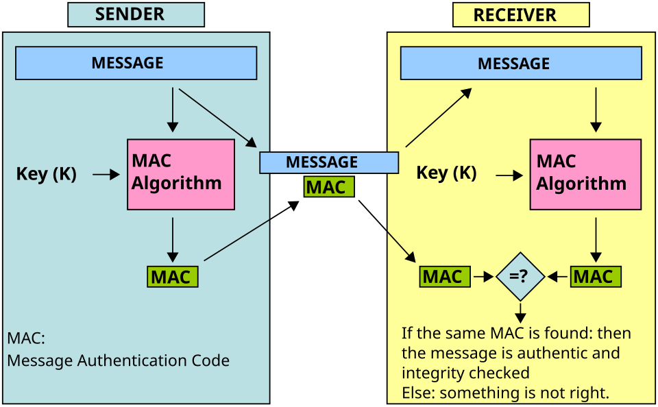
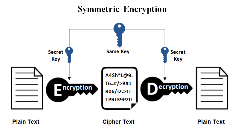
Symmetric Cryptography
covers MAC, secret key systems, and symmetric ciphers
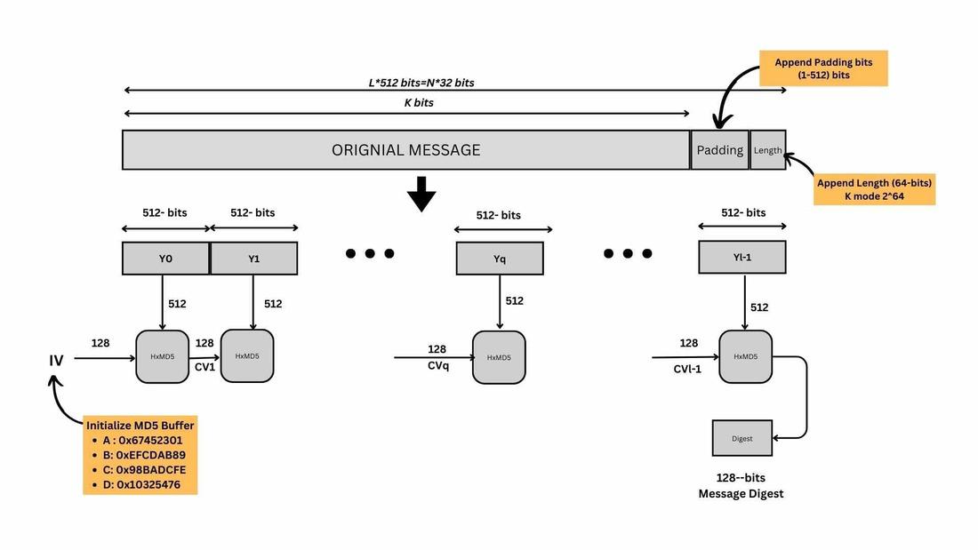
Hash Functions
Hash function uses in cryptographic schemes (no keys)
Public-Key Encryption
RSA, ECC, and ElGamal encryption schemes
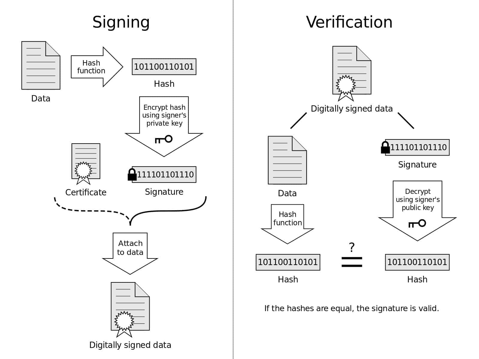
Digital Signatures & Authentication
Public-key authentication protocols, RSA signatures, and mutual authentication

Number Theory
Number theory in cypto - Euclidean algorithm, number factorization, modulo operations
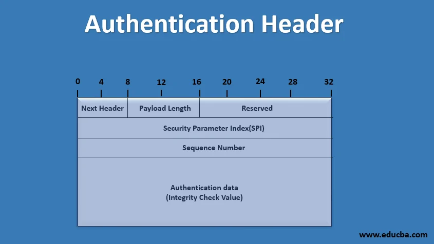
IPSec Types & Properties
Authentication Header (AH), ESP, Transport vs Tunnel modes