
Anatomy of Machine Learning
Machine Learning (ML) is the study of algorithms that enable systems to learn patterns from data and make predictions or decisions without being explicitly programmed for every case. This note provides a comprehensive overview of the theoretical, mathematical, and practical building blocks of modern ML.
Core Components of Machine Learning
- Data: The foundation of ML. Data may be structured (tabular), unstructured (text, images, audio), or multimodal.
- Model: A parameterized function that maps inputs to outputs. Examples include linear models, neural networks, and decision trees.
- Loss Function: Quantifies how far predictions are from ground truth.
- Optimizer: Algorithm that updates parameters to minimize the loss (e.g., Gradient Descent, Adam).
- Evaluation Metric: External measure of success (e.g., accuracy, F1 score, RMSE).
Theoretical Foundations: The Learning Problem
The central task in supervised machine learning is to learn a function $f: \mathcal{X} \to \mathcal{Y}$ from a dataset of input-output pairs $(\mathbf{x}, y) \in (\mathcal{X}, \mathcal{Y})$. The goal is to find a function $f^*$ from a hypothesis space $\mathcal{H}$ that minimizes the **expected risk** or **generalization error**, defined as:
where $P(\mathbf{x}, y)$ is the unknown true data distribution. Since we cannot calculate this directly, we approximate it using the **empirical risk** or **training error** over a finite dataset $\mathcal{D} = \{(\mathbf{x}_i, y_i)\}_{i=1}^N$:
The field of **statistical learning theory** provides a framework for understanding the relationship between empirical risk and expected risk, exploring the conditions under which a model that performs well on training data will also generalize to unseen data. Key concepts include **VC dimension** and the **bias-variance tradeoff**.
Perceptron & Multilayer Perceptrons (MLPs)
The perceptron is a binary linear classifier. For an input vector $\mathbf{x}$, the output is given by:
An MLP extends this to multiple layers, where each layer's output is a matrix-vector product followed by an element-wise non-linear activation function. For a single hidden layer, the output is:
where $\mathbf{W}$ are weight matrices, $\mathbf{b}$ are bias vectors, and $\sigma$ is the activation function. The **Universal Approximation Theorem** states that a single hidden layer MLP with a non-linear activation can approximate any continuous function to an arbitrary degree of accuracy, provided it has enough neurons.
Parameters in Standard MLP"; echo "Parameters = (weights + biases) per layer. Weights connect neurons between layers, biases allow shifting of activation thresholds.
"; echo "- ";
for ($i = 0; $i < count($layers) - 1; $i++) {
$input_nodes = $layers[$i];
$output_nodes = $layers[$i + 1];
$weights = $input_nodes * $output_nodes;
$biases = $output_nodes;
$layer_params = $weights + $biases;
$total += $layer_params;
echo "
- Layer " . ($i+1) . ": $input_nodes → $output_nodes | Weights ($weights) + Biases ($biases) = $layer_params "; } echo "
Total parameters: $total
"; } // Example usage: $layers = [784, 128, 64, 10]; mlp_parameters_explained($layers); ?>MLP Parameters
(#inputs * #hidden + #outputs) * (#hidden + 1) = (N + 1) * M
Accounts for weights and biases connecting input → hidden → output layers.
CNN Output Size
n_out = (N + 2p - k)/s + 1
- N: input size
- p: padding
- k: kernel size
- s: stride
CNN Parameters
Params = (C * k² + 1) * M
- C: number of input channels
- k²: kernel size squared
- M: number of filters
Loss vs. Activation Functions
- Activation Functions: Introduce non-linearity.
- Sigmoid ($\sigma(z) = 1 / (1 + e^{-z})$): Suffers from **vanishing gradients** when inputs are large or small, as its derivative approaches zero.
- ReLU ($f(x) = \max(0, x)$): The derivative is 1 for positive inputs, avoiding vanishing gradients. However, it can lead to "dead neurons" if inputs are always negative.
- GELU ($f(x) = x \cdot \Phi(x)$): A smoother, more complex function that is gaining popularity in modern architectures like Transformers.
- Loss Functions:
- For Regression:
- MSE (Mean Squared Error): For regression. Calculates the average of the squared differences between predicted and actual values. The loss is given by $\mathcal{L}_{\text{MSE}} = \frac{1}{N} \sum (y_i - \hat{y}_i)^2$.
- MAE (Mean Absolute Error): For regression. Calculates the average of the absolute difference between predicted and actual values. The loss is given by $\mathcal{L}_{\text{MSE}} = \frac{1}{N} \sum |y_i - \hat{y}_i|^2$. Unlike MSE, MAE gives equal weight to all errors. It's more robust to outliers since it doesn't square the errors. However, its derivative is not continuous at zero, which can make it difficult for gradient-based optimization algorithms to find the exact minimum.
- Huber Loss (Smooth MAE): This loss function combines the best of both worlds. It behaves like MSE for small errors and like MAE for large errors. It's often used when you need to be less sensitive to outliers than MSE but still want a smooth function near the minimum.
<li><b>For Classification:</b></li>
    <li><b>Cross-Entropy:</b> The standard loss for classification. It measures the performance of a classification model whose output is a probability value between 0 and 1. It's designed to heavily penalize models that are very confident but wrong.
        For binary classification, it is:
    <div class="equation">
        $$
        \mathcal{L}_{\text{BCE}} = -[y \log(\hat{y}) + (1-y) \log(1-\hat{y})]
        $$
    </div>
    <br> For multi-class classification, use categorical Cross-Entropy

    <li><b> Hinge Loss: </b>This loss function is particularly associated with Support Vector Machines (SVMs). It's used for binary classification and is designed to create a "margin" of separation between classes. </li>
    <li><b>One-Hot Encoding</b> Ground-truth labels represented as binary vectors with a 1 at the true class index. So bad, usually just used for preprocessing these days</li>
    <li> <b> Softmax: </b>Often used as activaton function with cross-entropy. Converts logits into probabilities,  converts a vector of raw prediction scores (called logits) into a probability distribution. Output vector sums to 1. Each element represents probability of class
        <!-- <div class="equation">
        $$
        \mathcal{p}_{\text{i}} = [y \log(\hat{y}) + (1-y) \log(1-\hat{y})]
        $$
    </div> -->
i.
Gradient Descent & Optimization: The Core of Training
The process of finding optimal model parameters $\theta$ is an iterative minimization problem. We update the parameters in the direction of the steepest decrease of the loss function, which is given by the negative of its gradient $\nabla_{\theta}\mathcal{L}(\theta)$. The update rule is:
where $\alpha$ is the learning rate, controlling the step size.
- Mini-batch GD: The gradient is computed over a small, random subset of the data. This provides a good balance between the computational efficiency of SGD and the stable convergence of Batch GD.
- Uses small subsets of data per iteration.
- Pros: balances efficiency and stability, commonly used in practice.
- Batch Gradient Descent (BGD)
- Uses all samples per iteration.
- Pros: stable convergence. Cons: slow, high memory cost.
- Stochastic Gradient Descent (SGD)
- Uses one sample per iteration.
- Pros: faster updates, can escape local minima.
- Cons: noisy updates, less stable.
- Momentum: Adds a fraction of the previous update vector to the current one, helping to smooth out oscillations and accelerate convergence in the right direction.
- Adam (Adaptive Moment Estimation): Combines momentum with a per-parameter adaptive learning rate based on the first and second moments of the gradients. This makes it highly effective and is a default choice for many tasks.
Overfitting vs Underfitting: The Bias-Variance Tradeoff
- High Bias (Underfitting): The model is too simple and fails to capture the underlying patterns in the data, leading to high errors on both training and test sets.
- High Variance (Overfitting): The model is too complex and fits the noise in the training data, leading to very low training error but high test error.
Regularization techniques are mathematical tools to combat overfitting by adding a penalty term to the loss function that discourages overly complex models. They are essential for ensuring that a model generalizes well to unseen data rather than just memorizing the training set.
- L2 Regularization (Weight Decay): Adds a term to the loss function that is proportional to the sum of the squared weights.$$ \mathcal{L}_{total} = \mathcal{L}_{original} + \lambda \sum_{i} \theta_i^2 $$This penalty encourages the model to use smaller, more distributed weights. Intuitively, it prevents any single feature from having a disproportionately large influence, leading to a smoother, less complex model. The hyperparameter $\lambda$ controls the strength of the regularization.
- L1 Regularization (Lasso): Adds a penalty term proportional to the sum of the absolute values of the weights.$$ \mathcal{L}_{total} = \mathcal{L}_{original} + \lambda \sum_{i} |\theta_i| $$Unlike L2, L1 regularization can drive the weights of less important features all the way to zero. This has the effect of **feature selection**, creating a sparse model where only the most relevant features are used.
- Dropout: This is a popular technique for neural networks. During training, a fraction of neurons are randomly deactivated, or "dropped out," at each training step. This prevents neurons from co-adapting too much, as they can't rely on the presence of specific other neurons. It forces the network to learn more robust and redundant features, making it less sensitive to the specific features of the training data. At test time, all neurons are active, but their outputs are scaled by the dropout probability to maintain the same expected output magnitude as during training.
- Early Stopping: A simple yet effective regularization method. Training is stopped when the performance on a validation dataset begins to degrade, even if the training loss is still decreasing. This prevents the model from continuing to learn the noise in the training data, which is a hallmark of overfitting. It is based on the principle that the optimal point for generalization is often reached before the training loss is fully minimized.
- Data Augmentation: A powerful technique, especially for tasks involving images, text, or audio. It involves creating new, artificial training data by applying minor transformations to the existing data. For images, this might include rotating, flipping, or cropping them. For text, it could be paraphrasing or adding synonyms. By artificially increasing the size and diversity of the training set, the model is exposed to more variations, making it more robust and less likely to overfit to specific examples.
Computer Vision
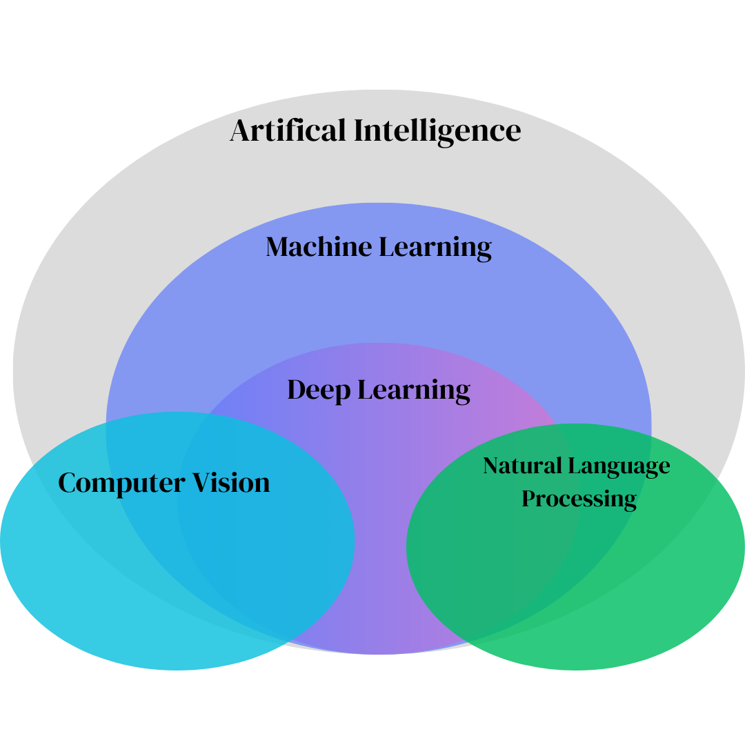
Overview of Computer Vision
Core concepts in computer vision and machine learning
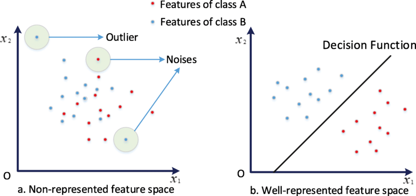
History of Computer Vision
How computer vision evolved through feature spaces
ImageNet Large Scale Visual Recognition Challenge
ImageNet's impact on modern computer vision
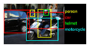
Region-CNNs
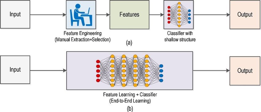
Traditional ML vs modern computer vision approaches
Distributed Systems
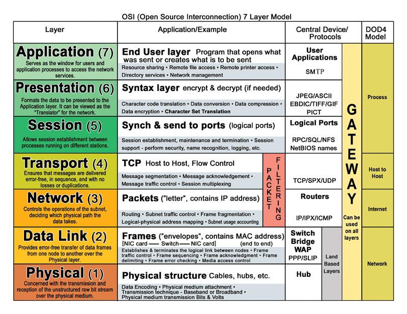
Overview of Distributed Systems
Fundamentals of distributed systems and the OSI model

Distributed Systems Architectures
Common design patterns for distributed systems
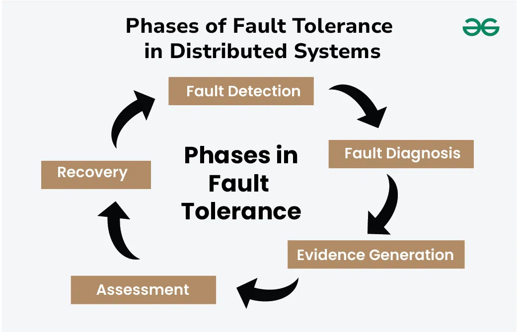
Dependability & Relevant Concepts
Reliability and fault tolerance in distributed systems
Marshalling
How data gets serialized for network communication
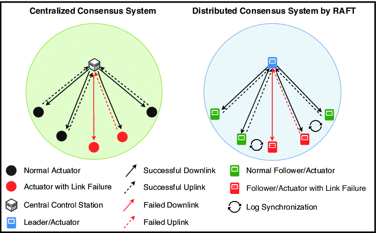
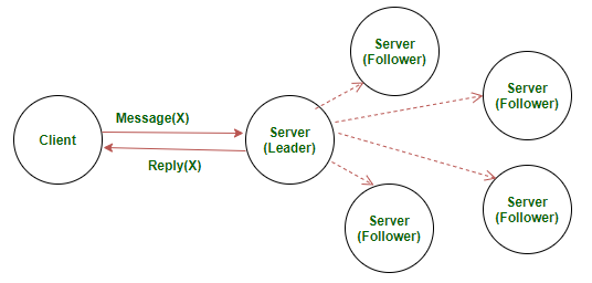
RAFT
Understanding the RAFT consensus algorithm
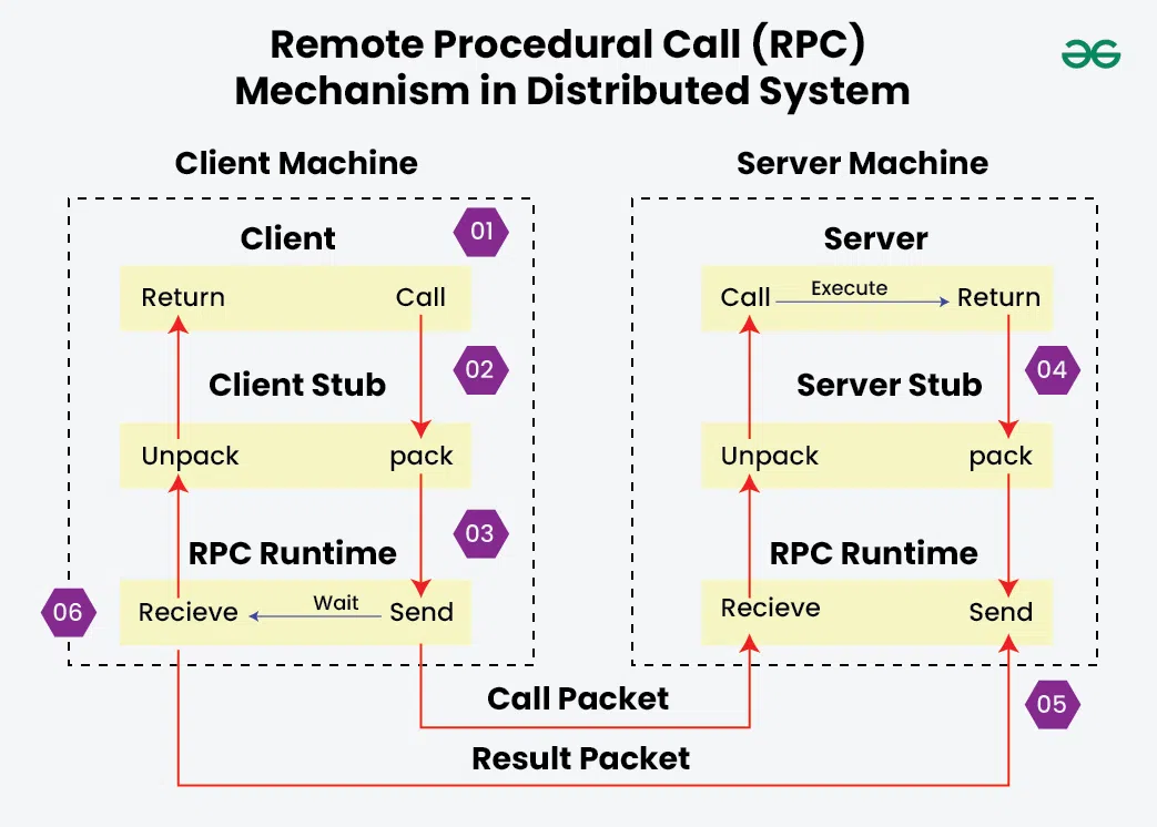
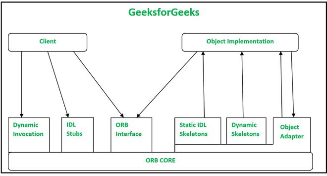
Remote Procedural Calls
How RPC enables communication between processes
Servers
Server design and RAFT implementation
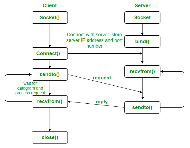
Sockets
Network programming with UDP sockets
Machine Learning (Generally Neural Networks)
Anatomy of Neural Networks
Traditional ML vs modern computer vision approaches

LeNet Architecture
The LeNet neural network
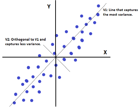
Principal Component Analysis
Explaining PCA from classical and ANN perspectives
Cryptography & Secure Digital Systems
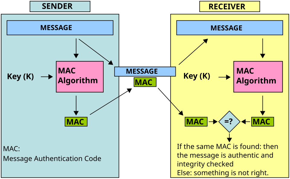
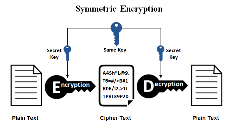
Symmetric Cryptography
covers MAC, secret key systems, and symmetric ciphers
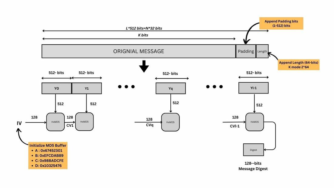
Hash Functions
Hash function uses in cryptographic schemes (no keys)
Public-Key Encryption
RSA, ECC, and ElGamal encryption schemes
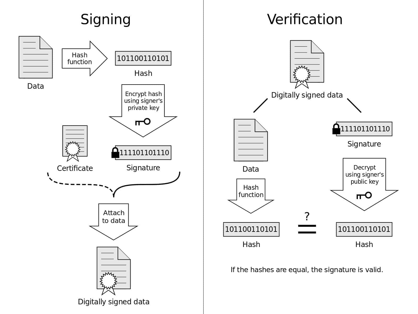
Digital Signatures & Authentication
Public-key authentication protocols, RSA signatures, and mutual authentication

Number Theory
Number theory in cypto - Euclidean algorithm, number factorization, modulo operations
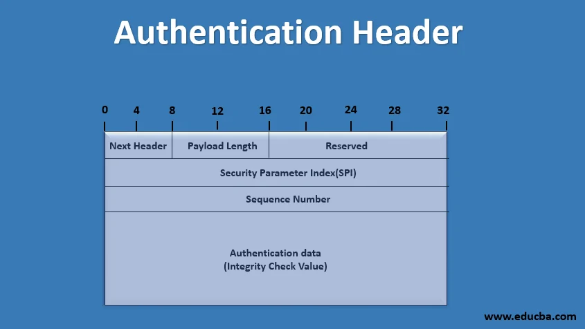
IPSec Types & Properties
Authentication Header (AH), ESP, Transport vs Tunnel modes